41 excel pivot table labels
› pivot-table-examplesPivot Table Examples | How to Create and Use the Pivot Table ... Though it is very flexible, Pivot Table has its limitations. You can’t make a change in the pivot table fields. You can’t add columns or rows under it and can’t add formula within the pivot table. If you wanted to make changes in a pivot table in a way not allowed normally, make a copy of your pivot table to some other sheet and then do. Repeat item labels in a PivotTable - support.microsoft.com Right-click the row or column label you want to repeat, and click Field Settings. Click the Layout & Print tab, and check the Repeat item labels box. Make sure Show item labels in tabular form is selected. Notes: When you edit any of the repeated labels, the changes you make are applied to all other cells with the same label.
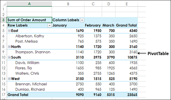
How to reset a custom pivot table row label Now go back to your Pivot and refresh it to find the Problem column and the duplicate column you just made. 5. Enter both fields into the pivot table and you will see the duplicate column has the original values while the Problem column maintains the problem labels. Monday, April 27, 2015 8:39 AM 0 Sign in to vote
Excel pivot table labels
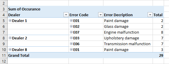
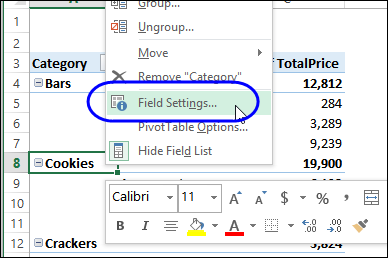
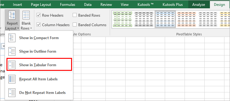
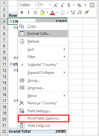
Repeat All Item Labels In An Excel Pivot Table | MyExcelOnline You can then select to Repeat All Item Labels which will fill in any gaps and allow you to take the data of the Pivot Table to a new location for further analysis. STEP 1: Click in the Pivot Table and choose PivotTable Tools > Options (Excel 2010) or Design (Excel 2013 & 2016) > Report Layouts > Show in Outline/Tabular Form Pivot Table "Row Labels" Header Frustration - Microsoft Community Hub Pivot Table "Row Labels" Header Frustration. Discussion Options. Janie1964. Occasional Visitor. Jul 28 2021 12:03 PM. › xlpivot05Fix Excel Pivot Table Missing Data Field Settings Aug 31, 2022 · For example, to include a new product -- Paper -- in the pivot table, even if it has not yet been sold: In the source data, add a record with Paper as the product, and 0 as the quantity; Refresh the pivot table, to update it with the new data; Right-click a cell in the Product field, and click Field Settings.
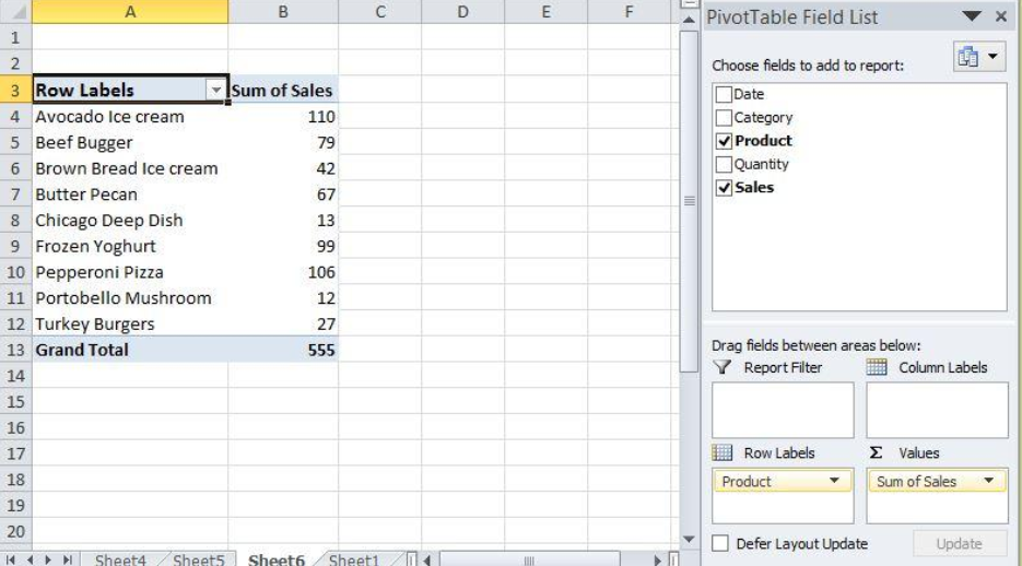
Excel pivot table labels. Pivot Table Row Labels - Microsoft Community If you go to PivotTable Tools > Analyze > Layout > Report Layout > Show in Tabular Form, your column headers will be used for the row labels. Every once in a while there's a sudden gust of gravity... Report abuse 1 person found this reply helpful · Was this reply helpful? Yes No A. User Replied on December 19, 2017 blog.hubspot.com › marketing › how-to-create-pivotHow to Create a Pivot Table in Excel: A Step-by-Step Tutorial Dec 31, 2021 · Every pivot table in Excel starts with a basic Excel table, where all your data is housed. To create this table, simply enter your values into a specific set of rows and columns. Use the topmost row or the topmost column to categorize your values by what they represent. Excel 2021 (Mac) - pivot tables - "Show items labels in tabular form" Just purchased Office 2021 (Mac) - on the PC version for pivot tables - in the "Field Settings", under the "Layout & Print" tab, there is a "Show items labels in tabular form" - is this function available in the Mac version - I cannot find it? If not is there anyway to accomplish the same via a different method on the Mac version Labels: PivotTable.RepeatAllLabels method (Excel) | Microsoft Learn Remarks. Using the RepeatAllLabels method corresponds to the Repeat All Item Labels and Do Not Repeat Item Labels commands on the Report Layout drop-down list of the PivotTable Tools Design tab. To specify whether to repeat item labels for a single PivotField, use the RepeatLabels property.
How to Use Excel Pivot Table Label Filters - Contextures Excel Tips Right-click a cell in the pivot table, and click PivotTable Options. In the PivotTable Options dialog box, click the Totals & Filters tab In the Filters section, add a check mark to 'Allow multiple filters per field.' Click the OK button, to apply the setting and close the dialog box. Quick Way to Hide or Show Pivot Items › excel-pivot-taHow to Create Excel Pivot Table (Includes practice file) Jun 28, 2022 · The area to the left results from your selections from [1] and [2]. You’ll see that the only difference I made in the last pivot table was to drag the AGE GROUP field underneath the PRECINCT field in the Row Labels quadrant. How to Create Excel Pivot Table. There are several ways to build a pivot table. › excel-pivot-table-formatHow to Format Excel Pivot Table - Contextures Excel Tips Jun 22, 2022 · Video: Change Pivot Table Labels. Watch this short video tutorial to see how to make these changes to the pivot table headings and labels. Get the Sample File. No Macros: To experiment with pivot table styles and formatting, download the sample file. The zipped file is in xlsx format, and and does NOT contain any macros. Remove row labels from pivot table • AuditExcel.co.za Click on the Pivot table. Click on the Design tab. Click on the report layout button. Choose either the Outline Format or the Tabular format. If you like the Compact Form but want to remove 'row labels' from the Pivot Table you can also achieve it by. Clicking on the Pivot Table. Clicking on the Analyse tab.
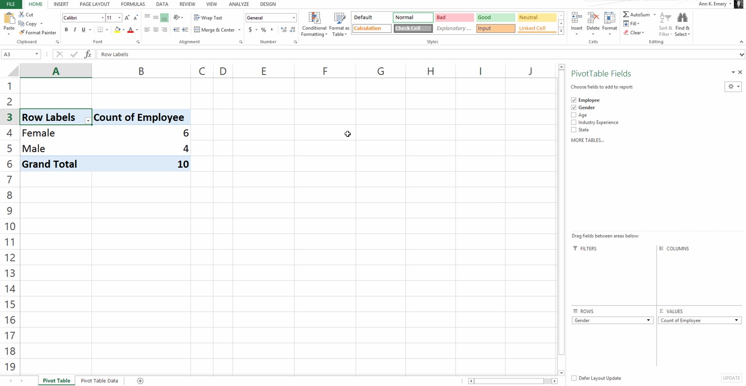
How to Use Label Filters for Text in the Pivot Table? To know how to create a Pivot table please Click Here. Step 2: To add a field, Tick the checkbox before the field name in the PivotTable Fields panel. When you select the field name, the selected field name will be inserted into the pivot table. Pro Tip. Row Labels are used to apply a filter to rows that have to be shown in the pivot table. › 2020/01/29 › hide-excel-pivotHide Excel Pivot Table Buttons and Labels Jan 29, 2020 · The field labels – Year, Region, and Cat – are hidden, and they weren’t really needed. The pivot table summary is easy to understand without those labels. NOTE: You can still sort and filter the pivot fields, if you right-click on a cell, and use the commands in the pop-up menu. More Pivot Table Tips. Go to my Contextures website for more ... How to unbold Pivot Table row labels | MrExcel Message Board Using Excel 2007, nested Pivot Table rows always seem to bold all but the inner-most row label. Is there a way to unbold all row labels? Displaying in Classic layout, tabular form, without expand/collapse buttons. Showing/Hiding subtotals doesn't seem to matter. I don't recall older versions (pre-2007) having this "feature." Design the layout and format of a PivotTable Change a PivotTable to compact, outline, or tabular form Change the way item labels are displayed in a layout form Change the field arrangement in a PivotTable Add fields to a PivotTable Copy fields in a PivotTable Rearrange fields in a PivotTable Remove fields from a PivotTable Change the layout of columns, rows, and subtotals
Pivot table row labels side by side – Excel Tutorial
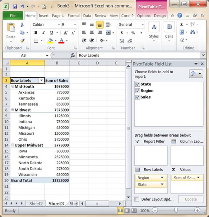
Automatic Row And Column Pivot Table Labels - How To Excel At Excel Select the data set you want to use for your table The first thing to do is put your cursor somewhere in your data list Select the Insert Tab Hit Pivot Table icon Next select Pivot Table option Select a table or range option Select to put your Table on a New Worksheet or on the current one, for this tutorial select the first option Click Ok
Centre Column Headings in Excel Pivot Table | Excel Pivot Tables
Excel 2016 Pivot table Row and Column Labels - Microsoft Community In Excel 2016 I've found when I create a pivot table it unhelpfully shows 'Row Labels' and 'Column Labels' instead of my field names, although in the top left cell it says 'Count of' and then inserts the correct field name. Years ago when I last used Excel it automatically put the field names in all three heading cells.
Repeat All Item Labels In An Excel Pivot Table | MyExcelOnline
Data Labels in Excel Pivot Chart (Detailed Analysis) 7 Suitable Examples with Data Labels in Excel Pivot Chart Considering All Factors 1. Adding Data Labels in Pivot Chart 2. Set Cell Values as Data Labels 3. Showing Percentages as Data Labels 4. Changing Appearance of Pivot Chart Labels 5. Changing Background of Data Labels 6. Dynamic Pivot Chart Data Labels with Slicers 7.
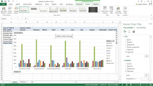
How to Customize Your Excel Pivot Chart and Axis Titles - dummies
Pivot table row labels in separate columns • AuditExcel.co.za Our preference is rather that the pivot tables are shown in tabular form (all columns separated and next to each other). You can do this by changing the report format. So when you click in the Pivot Table and click on the DESIGN tab one of the options is the Report Layout. Click on this and change it to Tabular form.
Turn Repeating Item Labels On and Off | Excel Pivot Tables
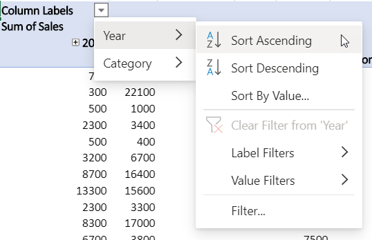
Excel: How to Sort Pivot Table by Date - Statology Often you may want to sort the rows in a pivot table in Excel by date. Fortunately this is easy to do using the sorting options in the dropdown menu within the Row Labels column of a pivot table. The following example shows exactly how to do so. Example: Sort Pivot Table by Date in Excel
Excel Pivot Tables - Sorting Data
How to Customize Your Excel Pivot Chart Data Labels - dummies The Data Labels command on the Design tab's Add Chart Element menu in Excel allows you to label data markers with values from your pivot table. When you click the command button, Excel displays a menu with commands corresponding to locations for the data labels: None, Center, Left, Right, Above, and Below.
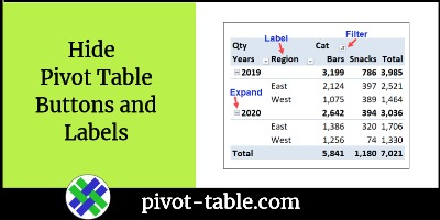
Hide Excel Pivot Table Buttons and Labels | Excel Pivot Tables
Pivot table row labels side by side - Excel Tutorial - OfficeTuts Excel You can copy the following table and paste it into your worksheet as Match Destination Formatting. Now, let's create a pivot table ( Insert >> Tables >> Pivot Table) and check all the values in Pivot Table Fields. Fields should look like this. Right-click inside a pivot table and choose PivotTable Options…. Check data as shown on the image below.
How to make row labels on same line in pivot table?
How to Move Excel Pivot Table Labels Quick Tricks - Contextures Excel Tips To move a pivot table label to a different position in the list, you can use commands in the right-click menu: Right-click on the label that you want to move Click the Move command Click one of the Move subcommands, such as Move [item name] Up The existing labels shift down, and the moved label takes its new position. Type Over Another Label

Remove Group Heading Excel Pivot Table - Stack Overflow
› xlpivot05Fix Excel Pivot Table Missing Data Field Settings Aug 31, 2022 · For example, to include a new product -- Paper -- in the pivot table, even if it has not yet been sold: In the source data, add a record with Paper as the product, and 0 as the quantity; Refresh the pivot table, to update it with the new data; Right-click a cell in the Product field, and click Field Settings.
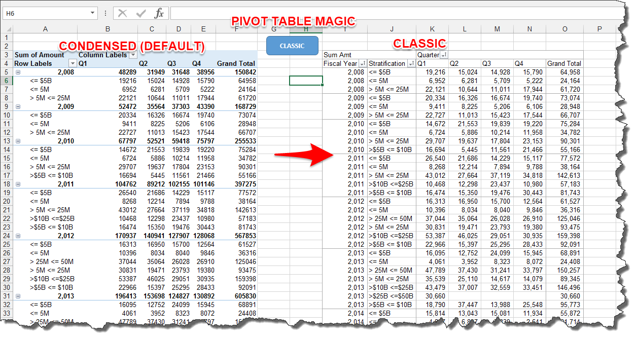
Microsoft Excel — Pivot Table Magic | by Don Tomoff | Let's ...
Pivot Table "Row Labels" Header Frustration - Microsoft Community Hub Pivot Table "Row Labels" Header Frustration. Discussion Options. Janie1964. Occasional Visitor. Jul 28 2021 12:03 PM.

Repeat item labels in a PivotTable
Repeat All Item Labels In An Excel Pivot Table | MyExcelOnline You can then select to Repeat All Item Labels which will fill in any gaps and allow you to take the data of the Pivot Table to a new location for further analysis. STEP 1: Click in the Pivot Table and choose PivotTable Tools > Options (Excel 2010) or Design (Excel 2013 & 2016) > Report Layouts > Show in Outline/Tabular Form
Design the layout and format of a PivotTable

Microsoft Excel Pivot Tables - Excel Consultant
Pivot Table shows row labels instead of field name

Excel Tips: Repeat Row Labels in Excel 2007
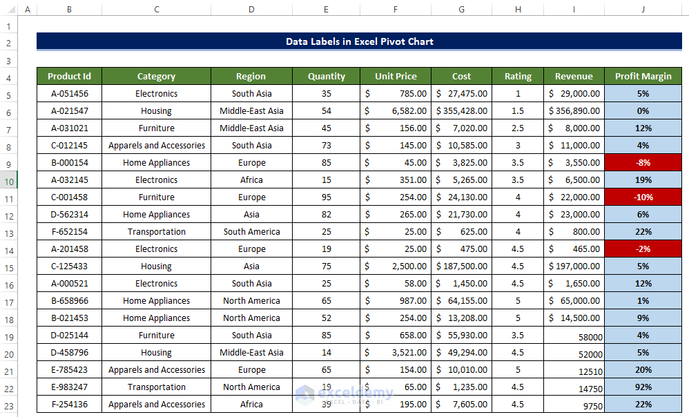
Data Labels in Excel Pivot Chart (Detailed Analysis) - ExcelDemy

Excel Pivot Tables | Pivot table, Excel, Table labels
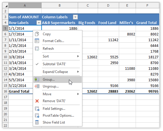
Group Items in a Pivot Table | DevExpress End-User Documentation
Excel PivotTable Percentage: Which Customers Are Costing You ...

Repeat all item labels in Pivot Table (aka Fill in the blanks ...

Pivot table row labels in separate columns • AuditExcel.co.za
Get Started with this Illustrated Pivot Table Tutorial ...
How to Save Time and Energy by Analyzing Your Data with Pivot ...
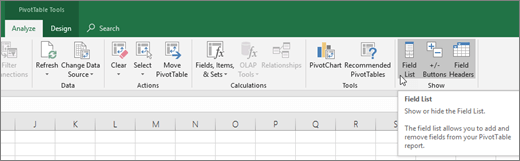
Use the Field List to arrange fields in a PivotTable
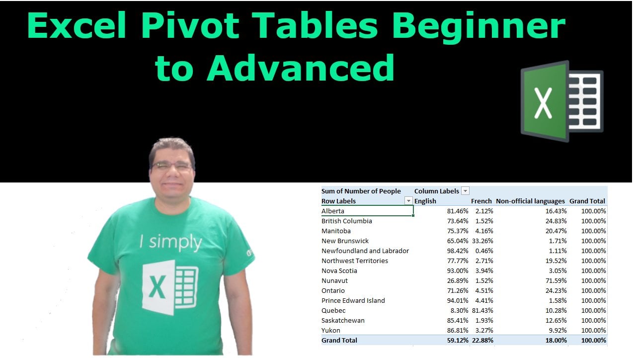
Excel Pivot Tables - Beginners to Advanced! Your ultimate ...

Repeat all item labels in Pivot Table (aka Fill in the blanks ...
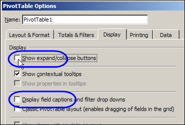
Hide Pivot Table Buttons and Labels – Contextures Blog
Pivot table row labels side by side – Excel Tutorial

MS Excel Pivot Table Deleted Items Remain - Excel and Access
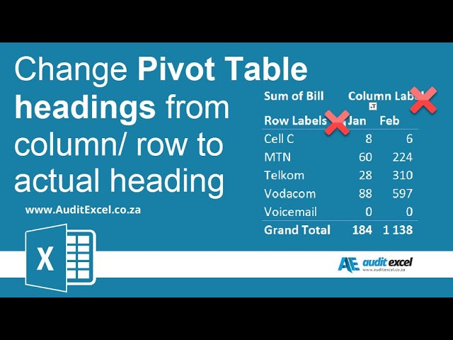
Pivot Table headings that say column/ row instead of actual ...

Working with Pivot Tables | Excel library | Syncfusion

Repeat Pivot Table row labels • AuditExcel.co.za Pivot Tables ...

How to Use Excel Pivot Table Label Filters

Change Pivot Table Sum of Headings and Blank Labels - YouTube

Fix Excel Pivot Table Missing Data Field Settings
How to make row labels on same line in pivot table?

Pivot table row labels side by side – Excel Tutorial
Excel Pivot Tables Explained • My Online Training Hub

Pivot Table Defaults to Count Instead of Sum & How to Fix It ...
Design the layout and format of a PivotTable

Pivot Table column label from horizontal to vertical ...
Post a Comment for "41 excel pivot table labels"