43 excel chart change labels

How to Create a Run Chart in Excel (2021 Guide) | 2 Free ... Download this Excel run chart template with dynamic data labels. Note: Since your median is going to be different, you need to adapt the custom number formatting accordingly ( Format Data Labels > Label Options > Number > Format Code > In the " Format Code " field, replace " 80 " with your median value as shown below). How to Add Axis Titles in a Microsoft Excel Chart Select your chart and then head to the Chart Design tab that displays. Click the Add Chart Element drop-down arrow and move your cursor to Axis Titles. In the pop-out menu, select "Primary Horizontal," "Primary Vertical," or both. If you're using Excel on Windows, you can also use the Chart Elements icon on the right of the chart.

How to Change the Y Axis in Excel - Alphr Click the dropdown next to "Display Units," then make your selection such as "millions" or "hundreds." To label the displayed units, go to the "Axis Options -> Display units" section. Add a...

Excel chart change labels

Modifying Axis Scale Labels (Microsoft Excel) Follow these steps: Create your chart as you normally would. Double-click the axis you want to scale. You should see the Format Axis dialog box. (If double-clicking doesn't work, right-click the axis and choose Format Axis from the resulting Context menu.) Make sure the Number tab is displayed. (See Figure 1.) Figure 1. How to Add Axis Label to Chart in Excel - Sheetaki Method 1: By Using the Chart Toolbar Select the chart that you want to add an axis label. Next, head over to the Chart tab. Click on the Axis Titles. Navigate through Primary Horizontal Axis Title > Title Below Axis. An Edit Title dialog box will appear. In this case, we will input "Month" as the horizontal axis label. Next, click OK. How to Format Excel Charts - Naukri Learning Change Axis Labels in a Chart. A label identifies each category on the horizontal axis. You can change the intervals at which these labels and minor tick marks appear. You can specify the location of the value (Y) axis to cross the category (X) axis on 2D charts. Right-click or double-click the category axis labels you need to format; Click Font

Excel chart change labels. Creating and Modifying Charts - Using Microsoft Excel ... In all cases, you have to select the chart first to access Chart Tools. To add any labels (for example, the title or axes), under the Design ribbon, click Add Chart Element in the Chart Layouts group and select the desired label. To change the chart type, data, or location, use the Chart Tools Design ribbon. Change The Font Size, Color, And Style Of An Excel Form ... So to change the Label's formatting — even when it's linked to the same cell — you'll need to click the label, click the formula bar, and retype the cell link. Admittedly, everyone else might have already figured this one out. However, I'm still very excited. Excel: How to Create a Bubble Chart with Labels - Statology The following labels will automatically be added to the bubble chart: Step 4: Customize the Bubble Chart. Lastly, feel free to click on individual elements of the chart to add a title, add axis labels, modify label font size, and remove gridlines: The final bubble chart is easy to read and we know exactly which bubbles represent which players. How to Use Excel Pivot Table Label Filters In an Excel pivot table, you might want to hide one or more of the items in a Row field or Column field. To do that, you could click the drop down arrow for the Row or Column Labels, then remove the check mark for items you want to remove. For example, to hide the data for 7-Feb-10, you'd click on the check mark to remove it.

Make better Excel Charts by adding graphics or pictures ... There's two ways to add images or graphics to an Excel chart. In this article we'll show how to overlay graphics over charts like the Pie Chart. In Better looking Excel Charts we'll show how to replace a colored chart block with an image. Insert picture into a chart . We have a basic 2D pie chart like this, very boring, very dull. Use defined names to automatically update a chart range ... On the Insert menu, click Chart to start the Chart Wizard. Click a chart type, and then click Next. Click the Series tab. In the Series list, click Sales. In the Category (X) axis labels box, replace the cell reference with the defined name Date. For example, the formula might be similar to the following: =Sheet1!Date How To Modify A Chart in Microsoft Excel? | Smart Office At the area of the ribbon and under the area named Type we have available the command Change Chart Type. If we are not satisfied with the Chart that we have created and we want to change it, we can use the command Change Chart Type. Once selected, the Change Chart Type dialog box appears as shown, with all the Charts available to use. How to format bar charts in Excel — storytelling with data 3. Click on any data label to highlight them all, then right-click and choose Format Data Labels: 4. In the Format Data Labels menu, select Label Options, and in the Label Positions section, choose Inside End. (While you're at it, in the Label Contains section, uncheck "Show Leader Lines.". These are almost never necessary.)

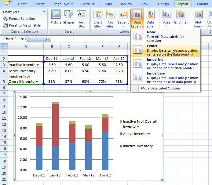
How to make shading on Excel chart and move x axis labels ... In the Change Chart Type dialog, change the chart type for the new series to Stacked Area. Change the color from whatever Excel decides to yellow. Finally, remove the new series form the legend. See the attached version. Wi-Fi Signal Strength.xlsx 15 KB 0 Likes Reply Snoopdon replied to Hans Vogelaar Oct 24 2021 05:18 PM Controlling Chart Gridlines (Microsoft Excel) When you create a chart from your data, Excel automatically takes care of many of the actual details related to how a specific chart appears. One of the elements that can be included on many of the charts is gridlines. Gridlines are helpful for easily determining the height or width of graphic elements used in your chart. How to Format Chart Axis to Percentage in Excel ... 2. Right-click on the axis. 3. Select the Format Axis option. 4. The Format Axis dialog box appears. In this go to the Number tab and expand it. Change the Category to Percentage and on doing so the axis data points will now be shown in the form of percentages. By default, the Decimal places will be of 2 digits in the percentage representation. Data label in the graph not showing percentage option ... Re: Data label in the graph not showing percentage option. only value coming. @Dipil. You need helper columns but you don't need another chart. Add columns with percentage and use "Values from cells" option to add it as data labels. labels percent.xlsx. Preview file.

Excel Dashboard Templates How-to Put Percentage Labels on Top of a Stacked Column Chart - Excel ...

Format Chart Axis in Excel - Axis Options (Format Axis ... However, In this blog, we will be working with Axis options, Tick marks, Labels, Number > Axis options> Axis options> Format Axis Pane. Axis Options: Axis Options There are multiple options So we will perform one by one. Changing Maximum and Minimum Bounds The first option is to adjust the maximum and minimum bounds for the axis.

How-to Use Data Labels from a Range in an Excel Chart - Excel Dashboard Templates

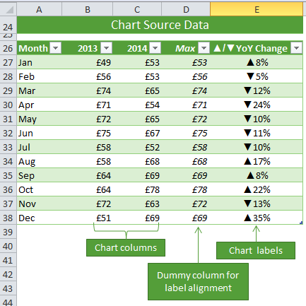
Custom Chart Data Labels In Excel With Formulas Follow the steps below to create the custom data labels. Select the chart label you want to change. In the formula-bar hit = (equals), select the cell reference containing your chart label's data. In this case, the first label is in cell E2. Finally, repeat for all your chart laebls.

5 Easy Steps to Make Your Excel Charts Look Professional | Easy-Excel.com

How to Change the X-Axis in Excel - Alphr Right-click the X-axis in the chart you want to change. That will allow you to edit the X-axis specifically. Then, click on Select Data. Select Edit right below the Horizontal Axis Labels tab....

Change Chart Data Labels : Chart Data « Chart « Microsoft Office Excel 2007 Tutorial

TickLabels object (Excel) | Microsoft Docs To change the tick-mark label text for the value axis, you must change the values of these properties. Example. Use the TickLabels property of the Axis object to return the TickLabels object. The following example sets the number format for the tick-mark labels on the value axis in embedded chart one on Sheet1.

Directly Labeling Excel Charts - PolicyViz

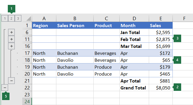
How to Move Excel Pivot Table Labels Quick Tricks Click on the cell where you want a different label to appear Type the name of the label that you want to move Press Enter The existing labels shift down, and the moved label takes its new position. For example, type "West" in cell A4, over the existing District name, "Central" Then, press Enter, to complete the change.

How to Make a Frequency Polygon in Excel - Statology

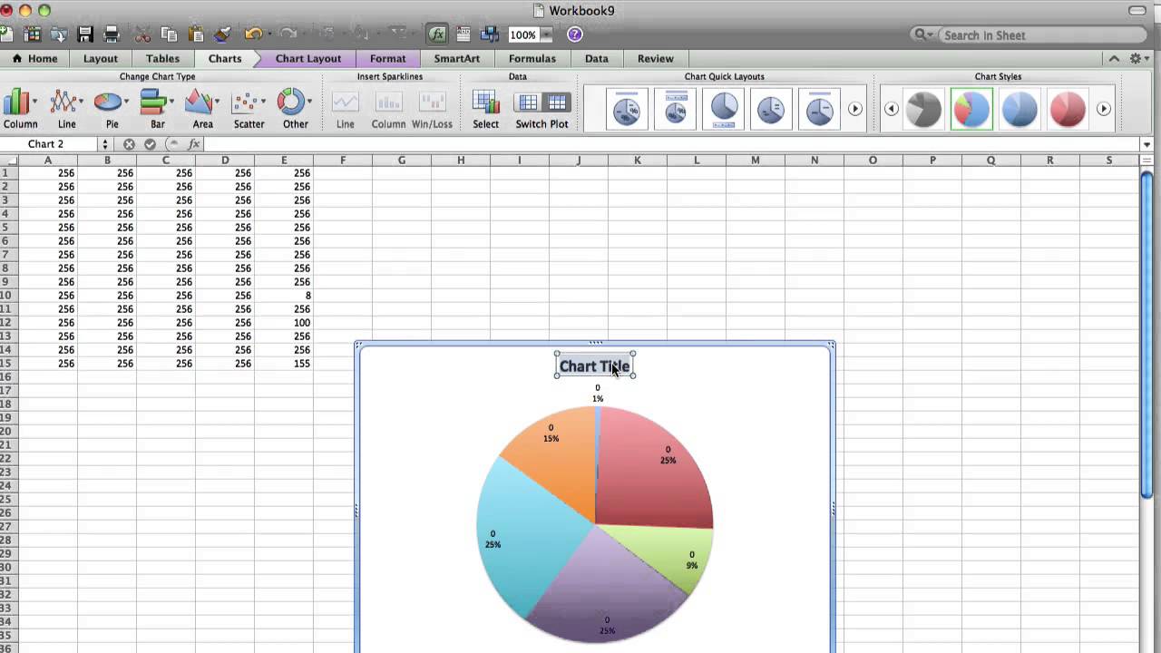
All About Chart Elements in Excel - Add, Delete, Change ... By default, Excel writes the text string "Chart Title" at the place of the chart title. We can rename the chart title by double-clicking on it. i.e "Monthly Sales" We can also change the position of the chart title by simply dragging it using the cursor. Download Above Image to Your Desktop >>>> Download Chart Data Labels

How to use symbols on charts in Excel

How to Print Labels from Excel - Lifewire Choose Start Mail Merge > Labels . Choose the brand in the Label Vendors box and then choose the product number, which is listed on the label package. You can also select New Label if you want to enter custom label dimensions. Click OK when you are ready to proceed. Connect the Worksheet to the Labels

Excel Chart Labeling - YouTube

How to Create and Customize a Waterfall Chart in Microsoft ... Select the chart and use the buttons on the right (Excel on Windows) to adjust Chart Elements like labels and the legend, or Chart Styles to pick a theme or color scheme. Select the chart and go to the Chart Design tab.

How to Change Excel Chart Name - YouTube

How to Add Labels to Scatterplot Points in Excel - Statology Step 3: Add Labels to Points Next, click anywhere on the chart until a green plus (+) sign appears in the top right corner. Then click Data Labels, then click More Options… In the Format Data Labels window that appears on the right of the screen, uncheck the box next to Y Value and check the box next to Value From Cells.

35 Label In Excel Definition - Labels Database 2020

How to Format Excel Charts - Naukri Learning Change Axis Labels in a Chart. A label identifies each category on the horizontal axis. You can change the intervals at which these labels and minor tick marks appear. You can specify the location of the value (Y) axis to cross the category (X) axis on 2D charts. Right-click or double-click the category axis labels you need to format; Click Font

Excel Course: Inserting Graphs

How to Add Axis Label to Chart in Excel - Sheetaki Method 1: By Using the Chart Toolbar Select the chart that you want to add an axis label. Next, head over to the Chart tab. Click on the Axis Titles. Navigate through Primary Horizontal Axis Title > Title Below Axis. An Edit Title dialog box will appear. In this case, we will input "Month" as the horizontal axis label. Next, click OK.